Thruster duty cycle#
We present an example using the duty-cycle functionality with Q-law. Specifically, we empose the thruster to abide by a duty-cycle, defined by a pair (ON,OFF), where ON denotes the maximum duration in time units (TU) over which the thruster can be used, and OFF denotes the duration required for the thruster to become usable again.
Note that this functionality does not allocate the use of the thruster optimally, but rather simply imposes a check with the duty-cycle on top of the existing Q-law mechanism.
We start with our usual imports
[1]:
import numpy as np
from numpy.random import rand
import matplotlib.pyplot as plt
import time

import sys
sys.path.append("../../../")    # only required if `pyqlaw` not installed
import pyqlaw
We now define our example going from GTO to GEO. The problem is solved using SMA-MEE.
[2]:
# initial and final elements: [a,e,i,RAAN,omega,ta]
LU = 42164.0
GM_EARTH = 398600.44
VU = np.sqrt(GM_EARTH/LU)
TU = LU/VU

rp_gto = 200 + 6378
ra_gto = 35786 + 6378
sma_gto = (rp_gto + ra_gto)/(2*LU)
ecc_gto = (ra_gto - rp_gto)/(ra_gto + rp_gto)
KEP0 = [sma_gto,ecc_gto,np.deg2rad(23),0,0,0]
KEPF = [1,0,np.deg2rad(3),0,0,0]

# initial and final elements with SMA-MEE
oe0 = pyqlaw.kep2mee_with_a(np.array(KEP0))
oeT = pyqlaw.kep2mee_with_a(np.array(KEPF))
woe = [3.0, 1.0, 1.0, 1.0, 1.0]
We define the duty-ratio; here, we consider a thruster that can fire for up to 85% of a day, after which it needs 15% of a day to cool down. The tuple duty_cycle is the ON and OFF times, in time units.
[3]:
# duty cycles
duty_cycle = (0.85*86400/TU, 0.15*86400/TU)
print(f"duty_cycle = {duty_cycle}")
duty_cycle = (5.355362190411142, 0.9450639159549075)
We define the spacecraft parameters, and canonicalize them.
[4]:
# spacecraft parameters
MU = 1200
tmax_si = 1            # Newtons
isp_si  = 1500         # seconds
mdot_si = tmax_si/(isp_si*9.81)  # kg/s

# non-dimensional quantities
mass0 = 1.0
tmax = tmax_si * (1/MU)*(TU**2/(1e3*LU))
mdot = np.abs(mdot_si) *(TU/MU)
tf_max = 10000.0
t_step = np.deg2rad(5)
We now assemble them into the problem object.
[5]:
# construct problem
prob = pyqlaw.QLaw(
    rpmin = 6578/LU,
    integrator="rk4",
    elements_type="mee_with_a",
    verbosity=2,
    print_frequency=3000,
    use_sundman = True,
)

# set problem
prob.set_problem(oe0, oeT, mass0, tmax, mdot, tf_max, t_step,
    duty_cycle = duty_cycle, woe=woe)
prob.pretty()
Transfer:
  a  : 5.7800e-01 -> 1.0000e+00 (weight: 3.00)
  f  : 7.3009e-01 -> 0.0000e+00 (weight: 1.00)
  g  : 0.0000e+00 -> 0.0000e+00 (weight: 1.00)
  h  : 2.0345e-01 -> 2.6186e-02 (weight: 1.00)
  k  : 0.0000e+00 -> 0.0000e+00 (weight: 1.00)
We can now solve the problem:
[6]:
# solve
prob.solve(eta_a=0.0, eta_r=0.2)
prob.pretty_results()
 iter   |  time      |  del1       |  del2       |  del3       |  del4       |  del5       |  el6        |
      0 |  1.039e-02 | -4.2200e-01 |  7.3009e-01 |  0.0000e+00 |  1.7727e-01 |  0.0000e+00 |  2.2018e-01 |
   3000 |  1.399e+02 | -2.1715e-01 |  4.6043e-01 |  5.5005e-03 |  3.4825e-02 |  1.1727e-03 |  2.6147e+02 |
Target elements successfully reached!
Exit code : 2
Converge  : True
Final state:
  a  : 9.9836e-01 (error: 1.6389e-03)
  f  : -1.2368e-03 (error: 1.2368e-03)
  g  : 7.7050e-03 (error: 7.7050e-03)
  h  : 2.6142e-02 (error: 4.4175e-05)
  k  : 4.7176e-04 (error: 4.7176e-04)
Transfer time : 293.89638400135607
Final mass    : 0.8622886035838151
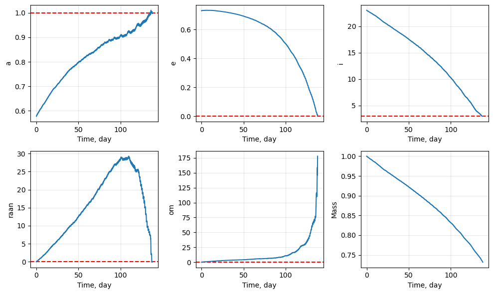
and visualize the results
[7]:
fig1, ax1 = prob.plot_elements_history(to_keplerian=True, TU=TU/86400, time_unit_name="day")
plt.show()
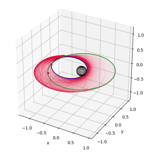
[8]:
fig2, ax2 = prob.plot_trajectory_3d(sphere_radius=6378/LU, lw=0.1, interpolate=False)
plt.show()
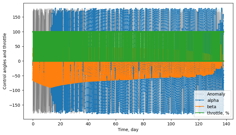
[9]:
fig3, ax3 = prob.plot_controls(TU=TU/86400, time_unit_name="day")
plt.show()
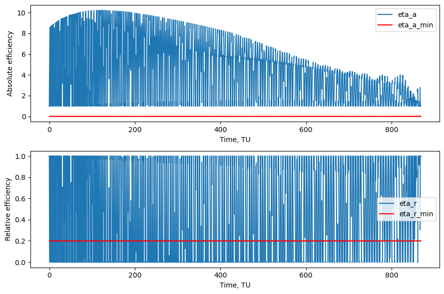
[10]:
fig4, ax4 = prob.plot_efficiency()
plt.show()
[ ]: