Pykep Compatible Problems#
The scocp_pykep extension provides OCP classes that are made to be compatible with pykep’s planet module to define initial/final rendez-vous conditions.
[!NOTE] Using the classes defined hereafter requires installing
scocp_pykepas well asscocp. In fact,scocp_pykephasscocpas one of its dependencies.
We consider a problem where:
the initial and final conditions are to rendez-vous with planets following Keplerian motion around the central body (a star);
the initial mass (wet mass) is fixed, and the objective is to maximize the final mass;
at departure and arrival, a v-infinity vector with a user-defined upper-bound on magnitude may be used;
the departure time from the initial planet and the arrival time are free and bounded;
This is analogous to `pykep.trajopt.direct_pl2pl <https://esa.github.io/pykep/documentation/trajopt.html#pykep.trajopt.direct_pl2pl>`__.
We will start with some imports
[1]:
import copy
import matplotlib.pyplot as plt
import numpy as np
from tqdm.auto import tqdm
import os
import sys

import pykep as pk

sys.path.append("../../..")    # path to scocp & scocp_pykep at the root of the repo
import scocp
import scocp_pykep
We now define our canonical scales.
[2]:
# define canonical parameters
GM_SUN = pk.MU_SUN           # Sun GM, m^3/s^-2
MSTAR  = 800.0               # reference spacecraft mass
G0     = pk.G0               # gravity at surface, m/s^2

DU = pk.AU                   # length scale set to Sun-Earth distance, m
VU = np.sqrt(GM_SUN / DU)    # velocity scale, m/s
TU = DU / VU                 # time scale, s
We will define the initial and final pykep.planet objects (here chosen to be Earth and Mars), the initial departure epoch bounds (defined in MJD), and the arrival time bounds (defined with respect to the initial )
[3]:
# define initial and final planets
pl0 = pk.planet.jpl_lp('earth')
plf = pk.planet.jpl_lp('mars')

t0_mjd2000_bounds = [1100.0, 1200.0]    # initial epoch in mjd2000
TU2DAY = TU / 86400.0                   # convert non-dimensional time to elapsed time in days

# define transfer problem discretization
tf_bounds = [1200.0, 1700.0]
t0_guess = 1100.0
tf_guess = 1600.0
N = 30
s_bounds = [0.01*tf_guess, 10*tf_guess]

# max v-infinity vector magnitudes
vinf_dep = 1e3/1e3     # 1000 m/s
vinf_arr = 500/1e3     # 500 m/s
[4]:
# spacecraft parameters
ISP    = 3000.0              # specific impulse, s
THRUST = 0.2                 # max thrust, kg.m/s^2

# this is the non-dimentional time integrator for solving the OCP
mu = GM_SUN / (VU**2 * DU)                          # canonical gravitational constant
c1 = THRUST / (MSTAR*DU/TU**2)                      # canonical max thrust
c2 = THRUST/(ISP*G0) / (MSTAR/TU)                   # canonical mass flow rate
print(f"Canonical mu: {mu:1.12e}, c1: {c1:1.4e}, c2: {c2:1.4e}")

ta_dyn, ta_dyn_aug = scocp_pykep.get_heyoka_integrator_twobody_mass(mu, c1, c2, tol=1e-15, verbose=True)
integrator_01domain = scocp_pykep.HeyokaIntegrator(
    nx=8,
    nu=4,
    nv=1,
    ta=ta_dyn,
    ta_stm=ta_dyn_aug,
    impulsive=False
)
Canonical mu: 1.000000000000e+00, c1: 4.2158e-02, c2: 4.2681e-02
Building integrator for state only ... Done! Elapsed time: 0.2748 seconds
Building integrator for state + STM ... Done! Elapsed time: 39.7368 seconds
Building the integrator is a timely procedure - but we can e.g. pickle the ta_dyn and ta_dyn_aug to speed this up:)
Construct a fuel-optimal problem#
We now construct the optimal control problem class for sequential convex programming corresponding to a rendezvous between two pykep.planet objects.
Let \(\boldsymbol{x}\) denote the state
and \(\boldsymbol{u}\) denote the control
where \(\| \boldsymbol{u} \|_2 = \Gamma \in [0,1]\).
The OCP we are solving is
To solve variable-time optimal control problems, we define \(\tau \in [0,1]\) such that the physical time \(t\) is a function \(t(\tau)\) satisfying \(t(0)=t_0\) and \(t(1) = t_f\). We define the augmented state \(\tilde{\boldsymbol{x}}\)
and augmented control \(\tilde{\boldsymbol{u}}\)
where \(s = \mathrm{d}t/\mathrm{d}\tau\). The controlled dynamics for the augmented state is given by
We formulate the fixed-time OCP in terms of the augmented state
Note: in the code, we denote \(\Gamma\) with v.
The corresponding OCP class is scocp_pykep.scocp_pl2pl.
Note that we set uniform_dilation = True, which makes the control segment duration equal, i.e. \(s_k = s_{k+1} \, \forall k\). This is found to result in more reliable convergence.
[5]:
# create problem
problem = scocp_pykep.scocp_pl2pl(
    integrator_01domain,
    pl0,
    plf,
    MSTAR,
    pk.MU_SUN,
    N,
    t0_mjd2000_bounds,
    tf_bounds,
    s_bounds,
    vinf_dep,
    vinf_arr,
    r_scaling = pk.AU,
    v_scaling = pk.EARTH_VELOCITY,
    uniform_dilation = True,
    objective_type = "mf",
)
The SCv* star algorithm needs an initial guess, which doesn’t need to be feasible. The scocp_pl2pl class provides a method for generating one by linearly interpolating between the initial and final orbital elements. Note that we could use any other way to generate some initial guess - and the “better” the initial guess is, the faster SCvx* will converge to a (hopefully better) local minimum - but of course that’s not trivial:)
[6]:
# create initial guess
xbar, ubar, vbar = problem.get_initial_guess(t0_guess, tf_guess)
ybar = np.zeros(6,)    # initial guess for v-infinity vectors
geq_nl_ig, sols_ig = problem.evaluate_nonlinear_dynamics(xbar, ubar, vbar, steps=5)   # evaluate initial guess
print(f"Max dynamics constraint violation: {np.max(np.abs(geq_nl_ig)):1.4e}")
Max dynamics constraint violation: 1.9342e+00
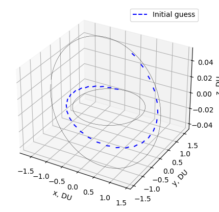
Let’s see what our initial guess trajectory looks like:
[7]:
# initial and final orbits
initial_orbit_states = problem.get_initial_orbit()
final_orbit_states = problem.get_final_orbit()

fig = plt.figure(figsize=(5,5))
ax = fig.add_subplot(1,1,1,projection='3d')
ax.set(xlabel="x, DU", ylabel="y, DU", zlabel="z, DU")
ax.plot(initial_orbit_states[1][:,0], initial_orbit_states[1][:,1], initial_orbit_states[1][:,2], 'k-', lw=0.3)
ax.plot(final_orbit_states[1][:,0], final_orbit_states[1][:,1], final_orbit_states[1][:,2], 'k-', lw=0.3)
for idx,(_ts, _ys) in enumerate(sols_ig):
    if idx == 0:
        label = "Initial guess"
    else:
        label = None
    ax.plot(_ys[:,0], _ys[:,1], _ys[:,2], '--', color='b', label=label)
ax.legend()
plt.show()
Solve fuel-optimal problem#
We can now solve the problem! We construct an instance of the SCvx* algorithm (scocp.SCvxStar), then call algo.solve(). Make sure that the feasibility tolerance (here set to tol_feas = 1e-12) is bigger than the integrator’s tolerance (using heyoka, we had set it to 1e-15).
[8]:
# setup algorithm & solve
tol_feas = 1e-12
tol_opt = 1e-6
algo = scocp.SCvxStar(problem, tol_opt=tol_opt, tol_feas=tol_feas, rho1=1e-8, r_bounds=[1e-10, 10.0])
solution = algo.solve(
    xbar,
    ubar,
    vbar,
    ybar=ybar,
    maxiter = 200,
    verbose = True
)
xopt, uopt, vopt, yopt, sols, summary_dict = solution.x, solution.u, solution.v, solution.y, solution.sols, solution.summary_dict
assert summary_dict["status"] == "Optimal"
assert summary_dict["chi"][-1] <= tol_feas
|  Iter  |     J0      |   Delta J   |   Delta L   |    chi     |     rho     |     r      |   weight   | step acpt. |
     1   | -6.0000e-01 |  1.2014e+02 |  1.1926e+02 | 1.7508e+00 |  1.0074e+00 | 1.0000e-01 | 1.0000e+02 |    yes     |
     2   | -4.0513e-01 |  6.6707e+02 |  6.6162e+02 | 1.1883e+00 |  1.0082e+00 | 3.0000e-01 | 2.0000e+02 |    yes     |
     3   | -9.1238e-01 |  6.1728e+02 |  6.5942e+02 | 5.3879e-01 |  9.3610e-01 | 9.0000e-01 | 2.0000e+02 |    yes     |
     4   | -1.1192e+00 |  5.4589e+01 |  1.0768e+02 | 9.0536e-01 |  5.0695e-01 | 2.7000e+00 | 2.0000e+02 |    yes     |
     5   | -9.1012e-01 |  5.0343e+02 |  5.3983e+02 | 1.2299e-01 |  9.3257e-01 | 2.7000e+00 | 4.0000e+02 |    yes     |
     6   | -1.0233e+00 |  3.2815e+01 |  3.6607e+01 | 1.3704e-01 |  8.9641e-01 | 8.1000e+00 | 4.0000e+02 |    yes     |
     7   | -9.8076e-01 | -1.5074e+02 |  2.6732e+01 | 2.2045e-01 | -5.6391e+00 | 1.0000e+01 | 8.0000e+02 |    no      |
     8   | -9.8076e-01 | -1.5074e+02 |  2.6732e+01 | 2.2045e-01 | -5.6392e+00 | 5.0000e+00 | 8.0000e+02 |    no      |
     9   | -9.8076e-01 | -1.5074e+02 |  2.6732e+01 | 2.2046e-01 | -5.6392e+00 | 2.5000e+00 | 8.0000e+02 |    no      |
    10   | -9.8076e-01 | -1.5074e+02 |  2.6732e+01 | 2.2046e-01 | -5.6392e+00 | 1.2500e+00 | 8.0000e+02 |    no      |

|  Iter  |     J0      |   Delta J   |   Delta L   |    chi     |     rho     |     r      |   weight   | step acpt. |
    11   | -9.2113e-01 | -2.0195e+01 |  2.6665e+01 | 9.9606e-02 | -7.5737e-01 | 6.2500e-01 | 8.0000e+02 |    no      |
    12   | -8.0011e-01 |  2.2655e+01 |  2.6525e+01 | 2.9513e-02 |  8.5410e-01 | 3.1250e-01 | 8.0000e+02 |    yes     |
    13   | -9.1664e-01 | -2.6649e+02 |  1.7593e+01 | 2.0205e-01 | -1.5148e+01 | 9.3750e-01 | 1.6000e+03 |    no      |
    14   | -8.7375e-01 | -3.0908e+01 |  1.7548e+01 | 7.5244e-02 | -1.7614e+00 | 4.6875e-01 | 1.6000e+03 |    no      |
    15   | -8.3565e-01 |  1.6248e+01 |  1.7509e+01 | 1.4414e-02 |  9.2800e-01 | 2.3438e-01 | 1.6000e+03 |    yes     |
    16   | -8.3476e-01 | -1.3318e+02 |  5.1706e+00 | 1.1921e-01 | -2.5756e+01 | 7.0312e-01 | 3.2000e+03 |    no      |
    17   | -8.3225e-01 | -2.5755e+01 |  5.1680e+00 | 4.9517e-02 | -4.9835e+00 | 3.5156e-01 | 3.2000e+03 |    no      |
    18   | -8.2598e-01 |  3.2964e+00 |  5.1620e+00 | 9.5506e-03 |  6.3858e-01 | 1.7578e-01 | 3.2000e+03 |    yes     |
    19   | -8.5044e-01 |  5.7589e-01 |  4.7244e+00 | 7.3733e-03 |  1.2190e-01 | 1.7578e-01 | 6.4000e+03 |    yes     |
    20   | -8.6124e-01 |  3.8856e-01 |  9.0381e+00 | 8.2036e-03 |  4.2992e-02 | 1.7578e-01 | 1.2800e+04 |    yes     |

|  Iter  |     J0      |   Delta J   |   Delta L   |    chi     |     rho     |     r      |   weight   | step acpt. |
    21   | -8.6196e-01 |  1.0240e+00 |  1.8020e+01 | 8.0302e-03 |  5.6824e-02 | 1.7578e-01 | 2.5600e+04 |    yes     |
    22   | -8.6436e-01 |  2.7243e+00 |  3.4431e+01 | 7.6529e-03 |  7.9124e-02 | 1.7578e-01 | 5.1200e+04 |    yes     |
    23   | -8.6593e-01 |  1.3332e-01 |  6.2646e+01 | 7.3862e-03 |  2.1281e-03 | 1.7578e-01 | 1.0240e+05 |    yes     |
    24   | -8.6318e-01 |  1.0717e+02 |  1.2672e+02 | 4.4721e-03 |  8.4574e-01 | 1.7578e-01 | 2.0480e+05 |    yes     |
    25   | -8.6062e-01 | -9.1653e+03 |  1.9545e+01 | 1.2601e-01 | -4.6894e+02 | 5.2734e-01 | 2.0480e+05 |    no      |
    26   | -8.5795e-01 | -6.1359e+02 |  1.9542e+01 | 2.5069e-02 | -3.1399e+01 | 2.6367e-01 | 2.0480e+05 |    no      |
    27   | -8.5646e-01 | -2.0257e+01 |  1.9541e+01 | 1.4816e-03 | -1.0367e+00 | 1.3184e-01 | 2.0480e+05 |    no      |
    28   | -8.5568e-01 |  1.7110e+01 |  1.9540e+01 | 5.5312e-03 |  8.7563e-01 | 6.5918e-02 | 2.0480e+05 |    yes     |
    29   | -8.7163e-01 | -4.0019e+02 |  2.2918e+01 | 1.7274e-02 | -1.7462e+01 | 1.9775e-01 | 4.0960e+05 |    no      |
    30   | -8.6968e-01 | -2.1494e+00 |  2.2916e+01 | 3.1902e-03 | -9.3794e-02 | 9.8877e-02 | 4.0960e+05 |    no      |

|  Iter  |     J0      |   Delta J   |   Delta L   |    chi     |     rho     |     r      |   weight   | step acpt. |
    31   | -8.6869e-01 |  2.1520e+01 |  2.2915e+01 | 2.6683e-04 |  9.3912e-01 | 4.9438e-02 | 4.0960e+05 |    yes     |
    32   | -8.6751e-01 | -9.5090e+01 |  1.4186e+00 | 5.1811e-03 | -6.7032e+01 | 1.4832e-01 | 8.1920e+05 |    no      |
    33   | -8.6704e-01 | -1.4178e+01 |  1.4181e+00 | 2.1273e-03 | -9.9979e+00 | 7.4158e-02 | 8.1920e+05 |    no      |
    34   | -8.6664e-01 |  4.7426e-01 |  1.4177e+00 | 1.9597e-04 |  3.3453e-01 | 3.7079e-02 | 8.1920e+05 |    yes     |
    35   | -8.6686e-01 | -3.7750e-01 |  9.8878e-01 | 3.1454e-04 | -3.8178e-01 | 3.7079e-02 | 1.6384e+06 |    no      |
    36   | -8.6680e-01 |  8.9800e-01 |  9.8871e-01 | 1.6392e-04 |  9.0825e-01 | 1.8539e-02 | 1.6384e+06 |    yes     |
    37   | -8.6711e-01 | -1.1932e+01 |  2.3918e-01 | 1.2722e-03 | -4.9887e+01 | 5.5618e-02 | 3.2768e+06 |    no      |
    38   | -8.6705e-01 | -6.1569e-01 |  2.3912e-01 | 2.7680e-04 | -2.5748e+00 | 2.7809e-02 | 3.2768e+06 |    no      |
    39   | -8.6702e-01 |  1.8087e-01 |  2.3909e-01 | 4.4208e-05 |  7.5650e-01 | 1.3905e-02 | 3.2768e+06 |    yes     |
    40   | -8.6720e-01 | -1.1833e+01 |  7.3247e-02 | 7.0007e-04 | -1.6155e+02 | 4.1714e-02 | 6.5536e+06 |    no      |

|  Iter  |     J0      |   Delta J   |   Delta L   |    chi     |     rho     |     r      |   weight   | step acpt. |
    41   | -8.6713e-01 | -7.5656e-01 |  7.3180e-02 | 1.5501e-04 | -1.0338e+01 | 2.0857e-02 | 6.5536e+06 |    no      |
    42   | -8.6709e-01 |  2.1174e-02 |  7.3145e-02 | 1.6458e-05 |  2.8948e-01 | 1.0428e-02 | 6.5536e+06 |    yes     |
    43   | -8.6712e-01 |  1.2316e-02 |  9.3265e-02 | 2.4774e-05 |  1.3205e-01 | 1.0428e-02 | 1.3107e+07 |    yes     |
    44   | -8.6716e-01 | -4.6222e-02 |  1.5165e-01 | 2.4652e-05 | -3.0481e-01 | 1.0428e-02 | 2.6214e+07 |    no      |
    45   | -8.6715e-01 |  1.3940e-01 |  1.5163e-01 | 1.2489e-05 |  9.1934e-01 | 5.2142e-03 | 2.6214e+07 |    yes     |
    46   | -8.6720e-01 | -1.5634e+00 |  4.2112e-03 | 8.6251e-05 | -3.7124e+02 | 1.5643e-02 | 5.2429e+07 |    no      |
    47   | -8.6718e-01 | -1.2160e-01 |  4.1900e-03 | 2.1615e-05 | -2.9021e+01 | 7.8213e-03 | 5.2429e+07 |    no      |
    48   | -8.6716e-01 | -3.5485e-03 |  4.1771e-03 | 7.6178e-07 | -8.4952e-01 | 3.9107e-03 | 5.2429e+07 |    no      |
    49   | -8.6716e-01 |  3.6876e-03 |  4.1707e-03 | 4.4575e-06 |  8.8417e-01 | 1.9553e-03 | 5.2429e+07 |    yes     |
    50   | -8.6718e-01 | -7.6964e-02 |  4.1607e-03 | 1.4768e-05 | -1.8498e+01 | 5.8660e-03 | 1.0486e+08 |    no      |

|  Iter  |     J0      |   Delta J   |   Delta L   |    chi     |     rho     |     r      |   weight   | step acpt. |
    51   | -8.6717e-01 | -8.4867e-04 |  4.1501e-03 | 3.0435e-06 | -2.0449e-01 | 2.9330e-03 | 1.0486e+08 |    no      |
    52   | -8.6716e-01 |  3.8377e-03 |  4.1448e-03 | 1.8394e-07 |  9.2590e-01 | 1.4665e-03 | 1.0486e+08 |    yes     |
    53   | -8.6718e-01 | -5.0832e-02 |  2.6826e-04 | 8.3057e-06 | -1.8949e+02 | 4.3995e-03 | 2.0972e+08 |    no      |
    54   | -8.6717e-01 | -2.8817e-03 |  2.6022e-04 | 1.7119e-06 | -1.1074e+01 | 2.1997e-03 | 2.0972e+08 |    no      |
    55   | -8.6717e-01 |  6.3488e-05 |  2.5619e-04 | 6.1578e-08 |  2.4781e-01 | 1.0999e-03 | 2.0972e+08 |    yes     |
    56   | -8.6717e-01 | -2.4183e-04 |  1.4672e-04 | 2.7569e-07 | -1.6482e+00 | 1.0999e-03 | 4.1943e+08 |    no      |
    57   | -8.6717e-01 |  1.2072e-04 |  1.4469e-04 | 1.3741e-07 |  8.3435e-01 | 5.4994e-04 | 4.1943e+08 |    yes     |
    58   | -8.6718e-01 | -4.0256e-03 |  1.8869e-05 | 1.1696e-06 | -2.1334e+02 | 1.6498e-03 | 8.3886e+08 |    no      |
    59   | -8.6717e-01 | -2.3284e-04 |  1.5782e-05 | 2.4144e-07 | -1.4753e+01 | 8.2491e-04 | 8.3886e+08 |    no      |
    60   | -8.6717e-01 | -1.0537e-06 |  1.4238e-05 | 8.8810e-09 | -7.4005e-02 | 4.1245e-04 | 8.3886e+08 |    no      |

|  Iter  |     J0      |   Delta J   |   Delta L   |    chi     |     rho     |     r      |   weight   | step acpt. |
    61   | -8.6717e-01 |  1.2514e-05 |  1.3464e-05 | 4.9502e-08 |  9.2942e-01 | 2.0623e-04 | 8.3886e+08 |    yes     |
    62   | -8.6717e-01 | -1.4887e-04 |  1.0362e-05 | 1.6524e-07 | -1.4367e+01 | 6.1868e-04 | 1.6777e+09 |    no      |
    63   | -8.6717e-01 | -6.2940e-07 |  9.1947e-06 | 3.4252e-08 | -6.8453e-02 | 3.0934e-04 | 1.6777e+09 |    no      |
    64   | -8.6717e-01 |  8.0028e-06 |  8.6104e-06 | 1.6701e-09 |  9.2944e-01 | 1.5467e-04 | 1.6777e+09 |    yes     |
    65   | -8.6717e-01 | -9.8509e-05 |  2.2445e-06 | 9.3166e-08 | -4.3890e+01 | 4.6401e-04 | 3.3554e+09 |    no      |
    66   | -8.6717e-01 | -4.8499e-06 |  1.3673e-06 | 1.9355e-08 | -3.5471e+00 | 2.3200e-04 | 3.3554e+09 |    no      |
    67   | -8.6717e-01 |  5.4492e-07 |  9.2823e-07 | 7.6734e-10 |  5.8705e-01 | 1.1600e-04 | 3.3554e+09 |    yes     |
    68   | -8.6717e-01 | -4.8605e-08 |  7.2696e-07 | 3.1875e-09 | -6.6861e-02 | 1.1600e-04 | 6.7109e+09 |    no      |
    69   | -8.6717e-01 |  4.5872e-07 |  5.0714e-07 | 1.5267e-09 |  9.0453e-01 | 5.8001e-05 | 6.7109e+09 |    yes     |
    70   | -8.6717e-01 | -7.2966e-06 |  6.8515e-07 | 1.3311e-08 | -1.0650e+01 | 1.7400e-04 | 1.3422e+10 |    no      |

|  Iter  |     J0      |   Delta J   |   Delta L   |    chi     |     rho     |     r      |   weight   | step acpt. |
    71   | -8.6717e-01 | -1.4601e-07 |  3.5531e-07 | 2.8055e-09 | -4.1094e-01 | 8.7002e-05 | 1.3422e+10 |    no      |
    72   | -8.6717e-01 |  1.5797e-07 |  1.8918e-07 | 1.2863e-10 |  8.3502e-01 | 4.3501e-05 | 1.3422e+10 |    yes     |
    73   | -8.6717e-01 | -4.6036e-06 |  5.2031e-07 | 7.5501e-09 | -8.8477e+00 | 1.3050e-04 | 2.6844e+10 |    no      |
    74   | -8.6717e-01 | -5.5861e-08 |  2.7238e-07 | 1.6035e-09 | -2.0509e-01 | 6.5251e-05 | 2.6844e+10 |    no      |
    75   | -8.6717e-01 |  1.2752e-07 |  1.4910e-07 | 2.1875e-10 |  8.5523e-01 | 3.2626e-05 | 2.6844e+10 |    yes     |
    76   | -8.6717e-01 | -2.8652e-06 |  3.9551e-07 | 4.2941e-09 | -7.2442e+00 | 9.7877e-05 | 5.3687e+10 |    no      |
    77   | -8.6717e-01 | -9.1764e-09 |  1.9977e-07 | 9.2078e-10 | -4.5936e-02 | 4.8938e-05 | 5.3687e+10 |    no      |
    78   | -8.6717e-01 |  9.9762e-08 |  1.1314e-07 | 4.8900e-11 |  8.8177e-01 | 2.4469e-05 | 5.3687e+10 |    yes     |
    79   | -8.6717e-01 | -1.8227e-06 |  2.8979e-07 | 2.4509e-09 | -6.2897e+00 | 7.3408e-05 | 1.0737e+11 |    no      |
    80   | -8.6717e-01 |  1.1611e-08 |  1.5007e-07 | 5.3204e-10 |  7.7370e-02 | 3.6704e-05 | 1.0737e+11 |    yes     |

|  Iter  |     J0      |   Delta J   |   Delta L   |    chi     |     rho     |     r      |   weight   | step acpt. |
    81   | -8.6717e-01 |  3.2320e-07 |  5.9606e-07 | 3.4786e-10 |  5.4222e-01 | 3.6704e-05 | 2.1475e+11 |    yes     |
    82   | -8.6717e-01 |  2.1141e-07 |  6.4914e-07 | 3.3308e-10 |  3.2567e-01 | 3.6704e-05 | 4.2950e+11 |    yes     |
    83   | -8.6717e-01 | -6.5343e-08 |  1.0323e-06 | 4.0269e-10 | -6.3298e-02 | 3.6704e-05 | 8.5899e+11 |    no      |
    84   | -8.6717e-01 |  8.8975e-07 |  9.7667e-07 | 1.8074e-10 |  9.1101e-01 | 1.8352e-05 | 8.5899e+11 |    yes     |
    85   | -8.6717e-01 | -1.1275e-05 |  3.5087e-07 | 1.4054e-09 | -3.2134e+01 | 5.5056e-05 | 1.7180e+12 |    no      |
    86   | -8.6717e-01 | -5.1184e-07 |  2.4541e-07 | 3.0979e-10 | -2.0856e+00 | 2.7528e-05 | 1.7180e+12 |    no      |
    87   | -8.6717e-01 |  1.3294e-07 |  1.9315e-07 | 2.0221e-11 |  6.8828e-01 | 1.3764e-05 | 1.7180e+12 |    yes     |
    88   | -8.6717e-01 | -1.7391e-08 |  1.0519e-07 | 5.8912e-11 | -1.6534e-01 | 1.3764e-05 | 3.4360e+12 |    no      |
    89   | -8.6717e-01 |  6.6954e-08 |  7.6095e-08 | 6.4937e-11 |  8.7988e-01 | 6.8820e-06 | 3.4360e+12 |    yes     |
    90   | -8.6717e-01 | -7.3369e-07 |  1.0465e-07 | 2.1655e-10 | -7.0109e+00 | 2.0646e-05 | 6.8719e+12 |    no      |

|  Iter  |     J0      |   Delta J   |   Delta L   |    chi     |     rho     |     r      |   weight   | step acpt. |
    91   | -8.6717e-01 | -2.8923e-10 |  5.9439e-08 | 4.8680e-11 | -4.8660e-03 | 1.0323e-05 | 6.8719e+12 |    no      |
    92   | -8.6717e-01 |  4.0862e-08 |  5.1179e-08 | 2.7143e-11 |  7.9842e-01 | 5.1615e-06 | 6.8719e+12 |    yes     |
    93   | -8.6717e-01 | -3.5465e-07 |  6.3779e-08 | 1.1975e-10 | -5.5606e+00 | 1.5484e-05 | 1.3744e+13 |    no      |
    94   | -8.6717e-01 | -1.2104e-08 |  5.2325e-08 | 3.3005e-11 | -2.3133e-01 | 7.7422e-06 | 1.3744e+13 |    no      |
    95   | -8.6717e-01 |  1.6958e-08 |  2.5522e-08 | 6.1197e-12 |  6.6443e-01 | 3.8711e-06 | 1.3744e+13 |    yes     |
    96   | -8.6717e-01 |  1.2097e-08 |  3.1393e-08 | 2.4169e-11 |  3.8535e-01 | 3.8711e-06 | 2.7488e+13 |    yes     |
    97   | -8.6717e-01 |  4.3505e-08 |  8.0304e-08 | 2.0864e-11 |  5.4176e-01 | 3.8711e-06 | 5.4976e+13 |    yes     |
    98   | -8.6717e-01 |  4.7334e-08 |  1.3450e-07 | 2.5307e-11 |  3.5193e-01 | 3.8711e-06 | 1.0995e+14 |    yes     |
    99   | -8.6717e-01 |  1.3888e-07 |  3.0334e-07 | 2.5107e-11 |  4.5783e-01 | 3.8711e-06 | 2.1990e+14 |    yes     |
   100   | -8.6717e-01 |  3.2921e-07 |  5.8709e-07 | 1.8135e-11 |  5.6075e-01 | 3.8711e-06 | 4.3980e+14 |    yes     |

|  Iter  |     J0      |   Delta J   |   Delta L   |    chi     |     rho     |     r      |   weight   | step acpt. |
   101   | -8.6717e-01 |  9.9142e-08 |  7.3739e-07 | 1.9760e-11 |  1.3445e-01 | 3.8711e-06 | 8.7961e+14 |    yes     |
   102   | -8.6717e-01 |  8.7703e-07 |  1.9082e-06 | 1.3132e-11 |  4.5960e-01 | 3.8711e-06 | 1.7592e+15 |    yes     |
   103   | -8.6717e-01 |  1.0090e-06 |  2.5275e-06 | 1.4608e-11 |  3.9921e-01 | 3.8711e-06 | 3.5184e+15 |    yes     |
   104   | -8.6717e-01 | -1.7637e-06 |  3.5056e-06 | 2.4555e-11 | -5.0311e-01 | 3.8711e-06 | 7.0369e+15 |    no      |
   105   | -8.6717e-01 |  2.1866e-06 |  3.4942e-06 | 3.1078e-12 |  6.2578e-01 | 1.9356e-06 | 7.0369e+15 |    yes     |
   106   | -8.6717e-01 | -6.0691e-07 |  1.4806e-06 | 1.2204e-11 | -4.0991e-01 | 1.9356e-06 | 1.4074e+16 |    no      |
   107   | -8.6717e-01 |  6.8874e-07 |  1.4768e-06 | 6.1007e-13 |  4.6637e-01 | 9.6778e-07 | 1.4074e+16 |    yes     |


    SCvx* algorithm summary:
        Status                          : Optimal
        Objective value                 : -8.67172738e-01
        Penalized objective improvement : 6.88741769e-07 (tol: 1.0000e-06)
        Constraint violation            : 6.10067552e-13 (tol: 1.0000e-12)
        Total iterations                : 107
        SCvx* algorithm time            : 25.4275 seconds
[9]:
problem.pretty(solution)
 ********* Trajectory summary *********
   Objective type       : mf
   Departure            : 1199.5133 MJD
   Arrival              : 1539.4673 MJD
   TOF                  : 439.4673 days
   Final mass           : 693.7382 kg
   Departure v-infinity : 1000.00 m/s
   Arrival v-infinity   : 500.00 m/s
[10]:
# evaluate nonlinear violations
geq_nl_opt, sols = problem.evaluate_nonlinear_dynamics(xopt, uopt, vopt, steps=4)
print(f"Max dynamics constraint violation: {np.max(np.abs(geq_nl_opt)):1.4e}")
assert np.max(np.abs(geq_nl_opt)) <= tol_feas
Max dynamics constraint violation: 3.5438e-13
[11]:
# extract solution
ts_mjd2000, states, controls, v_infinities = problem.process_solution(solution)
print(f"ts_mjd2000.shape = {ts_mjd2000.shape}")
print(f"states.shape = {states.shape}")
print(f"controls.shape = {controls.shape}")
ts_mjd2000.shape = (31,)
states.shape = (31, 7)
controls.shape = (30, 3)
In the above,
ts_mjd2000is a 1D array of the time-stamps of theN+1nodes in MJD,controlsis a 2D array containing the thrust throttles in each row for theNcontrol segments (remember we solved this via a stark model, i.e. constant thrust is applied across the segment),statesis a 2D array containing the cartesian state and mass of the spacecraft at the beginning of each node, andv_infinitiesis a list containing the initial and final v-infinity vectors
Plot results#
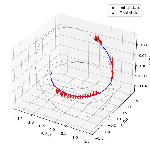
Let’s plot the results! Let’s first look at our controlled trajectory:
[12]:
# plot trajectory
x0 = problem.target_initial.target_state(xopt[0,7])
xf = problem.target_final.target_state(xopt[-1,7])

fig = plt.figure(figsize=(9,7))
ax = fig.add_subplot(1,1,1,projection='3d')
ax.set(xlabel="x", ylabel="y", zlabel="z")
for (_ts, _ys) in sols_ig:
    ax.plot(_ys[:,0], _ys[:,1], _ys[:,2], '--', color='grey')
for (_ts, _ys) in sols:
    ax.plot(_ys[:,0], _ys[:,1], _ys[:,2], 'b-')
    _us_zoh = scocp.zoh_controls(problem.times, uopt, _ts)
    ax.quiver(_ys[:,0], _ys[:,1], _ys[:,2], _us_zoh[:,0], _us_zoh[:,1], _us_zoh[:,2], color='r', length=0.05)

ax.scatter(x0[0], x0[1], x0[2], marker='x', color='k', label='Initial state')
ax.scatter(xf[0], xf[1], xf[2], marker='o', color='k', label='Final state')
ax.plot(initial_orbit_states[1][:,0], initial_orbit_states[1][:,1], initial_orbit_states[1][:,2], 'k-', lw=0.3)
ax.plot(final_orbit_states[1][:,0], final_orbit_states[1][:,1], final_orbit_states[1][:,2], 'k-', lw=0.3)
# ax.set_aspect('equal')
ax.set(xlabel="x, DU", ylabel="y, DU", zlabel="z, DU")
ax.legend()
plt.show()
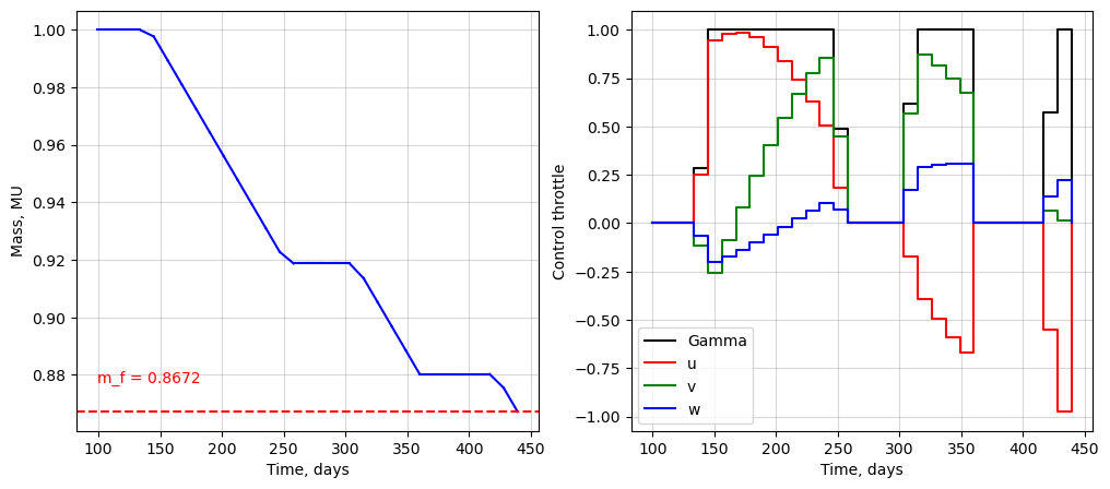
Let’s also look at the mass history and the control history:
[13]:
fig = plt.figure(figsize=(12,5))
ax_m = fig.add_subplot(1,2,1)
ax_m.grid(True, alpha=0.5)
for (_ts, _ys) in sols:
    ax_m.plot(_ys[:,7]*problem.TU2DAY, _ys[:,6], 'b-')
ax_m.axhline(sols[-1][1][-1,6], color='r', linestyle='--')
ax_m.text(xopt[0,7]*problem.TU2DAY, 0.01 + sols[-1][1][-1,6], f"m_f = {sols[-1][1][-1,6]:1.4f}", color='r')
ax_m.set(xlabel="Time, days", ylabel="Mass, MU")
#ax_m.legend()

ax_u = fig.add_subplot(1,2,2)
ax_u.grid(True, alpha=0.5)
ax_u.step(xopt[:,7]*problem.TU2DAY, np.concatenate((vopt[:,0], [0.0])), label="Gamma", where='post', color='k')
ax_u.step(xopt[:,7]*problem.TU2DAY, np.concatenate((uopt[:,0], [0.0])), label="u", where='post', color='r')
ax_u.step(xopt[:,7]*problem.TU2DAY, np.concatenate((uopt[:,1], [0.0])), label="v", where='post', color='g')
ax_u.step(xopt[:,7]*problem.TU2DAY, np.concatenate((uopt[:,2], [0.0])), label="w", where='post', color='b')
ax_u.set(xlabel="Time, days", ylabel="Control throttle")
ax_u.legend()
plt.show()
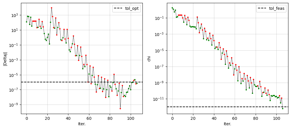
Let’s also see the convergence of the SCVx* algorithm - we will look at the iterates of \(|\Delta J|\), i.e. the actual cost reduction in a single SCP step, and \(\chi\), i.e. max nonlinear constraint violation at a given SCP step:
[14]:
fig = plt.figure(figsize=(12,5))
ax_DeltaJ = fig.add_subplot(1,2,1)
ax_DeltaJ.grid(True, alpha=0.5)
algo.plot_DeltaJ(ax_DeltaJ, summary_dict)
ax_DeltaJ.axhline(tol_opt, color='k', linestyle='--', label='tol_opt')
ax_DeltaJ.legend()

ax_DeltaL = fig.add_subplot(1,2,2)
ax_DeltaL.grid(True, alpha=0.5)
algo.plot_chi(ax_DeltaL, summary_dict)
ax_DeltaL.axhline(tol_feas, color='k', linestyle='--', label='tol_feas')
ax_DeltaL.legend()
plt.show()
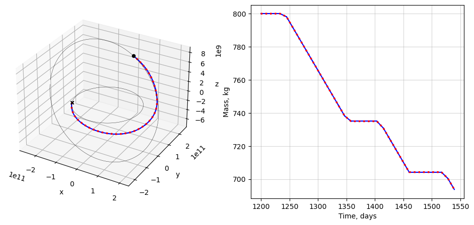
Verify the solution#
Let us now check if our constructed trajectory is dynamically feasible via forward single-shot propagation (remember: the dynamics was enforced in a multiple-shooting sence within the OCP). For this, we make use of pykep.propagate_taylor (from pykep 2.X) or pykep.stark_problem (from pykep 3.X).
[15]:
ts_mjd2000, states, controls, v_infinities = problem.process_solution(solution)
[16]:
x0_iter = states[0,0:7]     # initial spacecraft state
states_singleshoot = [x0_iter,]

for idx, (t0,u0) in tqdm(enumerate(zip(ts_mjd2000, controls)), total=len(controls)):
    r,v,m = pk.propagate_taylor(
        r0 = x0_iter[0:3],
        v0 = x0_iter[3:6],
        m0 = x0_iter[6],
        thrust = THRUST * np.array(u0),
        tof = (ts_mjd2000[idx+1] - ts_mjd2000[idx])*86400,
        mu = pk.MU_SUN,
        veff = ISP*G0,
        log10tol =-15,
        log10rtol = -15)

    # update spacecraft state
    x0_iter = np.concatenate((r,v,[m]))

    states_singleshoot.append(copy.deepcopy(x0_iter))
states_singleshoot = np.array(states_singleshoot)
[17]:
dx_final = states_singleshoot[-1,0:6] - np.concatenate(plf.eph(ts_mjd2000[-1]))  - np.concatenate((np.zeros(3), v_infinities[1]))
print(f"Final position offset: {dx_final[0:3]/1e3} km")
print(f"Final velocity offset: {dx_final[3:6]} m/s")
Final position offset: [-176.91088161  -30.19200256    1.14562381] km
Final velocity offset: [-0.00328417 -0.01671438 -0.00014991] m/s
[18]:
fig = plt.figure(figsize=(12,5))
ax = fig.add_subplot(1,2,1,projection='3d')
ax.set(xlabel="x", ylabel="y", zlabel="z")
for (_ts, _ys) in sols:
    ax.plot(_ys[:,0]*DU, _ys[:,1]*DU, _ys[:,2]*DU, 'b-', linewidth=1.5)
ax.plot(states_singleshoot[:,0], states_singleshoot[:,1], states_singleshoot[:,2], 'r:', linewidth=2.5)
ax.scatter(x0[0]*DU, x0[1]*DU, x0[2]*DU, marker='x', color='k', label='Initial state')
ax.scatter(xf[0]*DU, xf[1]*DU, xf[2]*DU, marker='o', color='k', label='Final state')
ax.plot(initial_orbit_states[1][:,0]*DU, initial_orbit_states[1][:,1]*DU, initial_orbit_states[1][:,2]*DU, 'k-', lw=0.3)
ax.plot(final_orbit_states[1][:,0]*DU, final_orbit_states[1][:,1]*DU, final_orbit_states[1][:,2]*DU, 'k-', lw=0.3)


axm = fig.add_subplot(1,2,2)
axm.grid(True, alpha=0.5)
axm.set(xlabel="Time, days", ylabel="Mass, kg")
for (_ts, _ys) in sols:
    axm.plot(problem.t0_min + _ys[:,7]*problem.TU2DAY, _ys[:,6]*MSTAR, 'b-', linewidth=1.5)
axm.plot(ts_mjd2000, states_singleshoot[:,6], 'r:', linewidth=2.5)
plt.show()
[ ]:
[ ]:
[ ]: